Have you ever written a program in Scratch or Python? You run it for the first time...

And it works perfectly.

Yeah. Me neither.

When a program gives you the wrong answer, you don't throw away the computer. You ask, where did the error come from? Maybe you made a typo. Maybe your equation was wrong. Maybe your logic made sense in your head but not in the program. You find the problem, change something, run it again, and see whether the result gets better.

That's debugging.

Scientists and engineers do something remarkably similar. We call it error analysis.

When you measure the acceleration of a cart, test the strength of a material, build a prototype, or run a chemical experiment, your result will almost never be exactly what a textbook equation predicts.

But here's the important part:

A difference between your result and the expected result does not automatically mean you did something wrong.

Maybe your measuring instrument isn't precise enough. Maybe your experimental conditions weren't exactly what you assumed. Maybe several small effects added together. Maybe your mathematical model was only an approximation. Or maybe you've discovered something interesting.

Error analysis gives you a way to tell the difference. Instead of simply asking, "Is my answer wrong?", scientists and engineers ask better questions:

• How far off is it?
• Why is it off?
• Can I quantify the uncertainty?
• Is the error random or systematic?
• Does it actually matter?
• What can the error teach me?

Engineers use error analysis to decide whether a structure is safe. Scientists use it to determine whether an experimental result is meaningful. And researchers use it to recognize when a result that looks like an error might actually be telling them something new.

Today, we're going to learn how to debug the physical world. Just like debugging a program, the goal isn't to eliminate every error. The goal is to understand what the errors are telling you.

• Measurement error: The difference between an actual, true value and the recorded or measured value
• Formulation & Modeling error: Mistakes when turning a real-world scenario into a math equation or model. For example, calculating a tip at a restaurant based on the total bill---including taxes.
• Numerical error: The difference between an exact mathematical value and the approximate value produced by a computer or calculation method. Some of the errors in this category include: roundoff, truncation, discretization.
• Data transmission & encoding errors: Noise along a transmission line, a corrupted file
• Algorithmic or logical error: My computer program has a bug or fails to account for some edge case.
• Human error: Blunders caused by human oversight, fatigue, or miscommunication.
• Interpretation error: Going to the gym, seeing "20" on a dumbbell and assuming it is 20 lbs when it's actually 20 kgs.
• Statistical error: Dissatisfied customers are more likely to leave reviews. Generally, only a small fraction of satisfied customers leave reviews. So if you see a 3-star review on Google Maps or Amazon, it's probably skewed negative. This is called selection bias in statistics.

For this class, we will focus mostly on measurement error and numerical error, but always keep in mind that errors can come from lots of different sources!

When you measure something in the real world, your measurement is never perfectly exact. Even if you measure the same object carefully, the result can change slightly depending on the tool you use, how you use it, and how precisely you can read it. The difference between the value you measure and the object's actual value is called measurement error.

Consider the pencil you just measured. With a ruler, you might report its diameter as 7 mm. But is it really exactly 7.000 mm? Probably not. A ruler has limited markings, your eyes have limited ability to judge between those markings, and you may not hold the ruler perfectly across the pencil. A set of calipers gives you much finer resolution, and the jaws are square to the object for better alignment. With calipers, you can make a more precise measurement—but even calipers aren't perfect.

This raises an important question: If two tools give you different measurements, which one is correct? The answer isn't necessarily the measurement with more digits. Measurement error is about understanding the limits of your measurement—including the tool, the technique, and the conditions under which you measured it. The better your understanding of those limits, the better you can judge how close your measurement is likely to be to the true value.

Learning about different representations of numbers will be useful when we talk about roundoff error in the next section.

• Binary numbers (Base 2). Uses two digits: 0 and 1. Example:

• Decimal numbers (Base 10). Uses ten digits: 0 through 9. Example:

How do you convert between the two? From binary to decimal, you can just use the definition above. For example, using the example above,

To go from decimal to binary, this video gives a good explanation of the steps:

Computers are really good at math—but they don't have infinite precision. A computer can only store numbers using a limited number of digits. When a number has more digits than the computer can keep, it has to round the number. The tiny difference between the number you wanted and the number the computer actually stored is called roundoff error.

For example, suppose you need to use the number π. You might use 3.141592653589793, but a calculation might store only some of those digits. The difference seems tiny—and usually it is. But here's the surprising part: tiny errors can sometimes add up. After thousands or millions of calculations, those little differences can accumulate and produce a result that is noticeably wrong.

Roundoff error is a reminder that even when your math is correct, the way a computer represents and calculates the numbers can introduce error. In numerical computing, part of the challenge isn't just getting the right equation—it's making sure the computer has enough precision to get a trustworthy answer. Sometimes, keeping the numbers in fractional form and using pencil and paper can give you a more accurate answer than a calculator or computer.

Sometimes we introduce error not because a computer can't represent a number accurately, but because we choose to stop a calculation early. This is called truncation error. Instead of carrying a calculation all the way to its exact result, we use an approximation that is easier or faster to calculate.

Truncation error shows up everywhere in science and engineering. We approximate complicated equations, replace continuous processes with small time steps in computer simulations, and simplify mathematical models so they can actually be calculated. The key idea is that truncation error comes from stopping an approximation process before reaching the exact result.


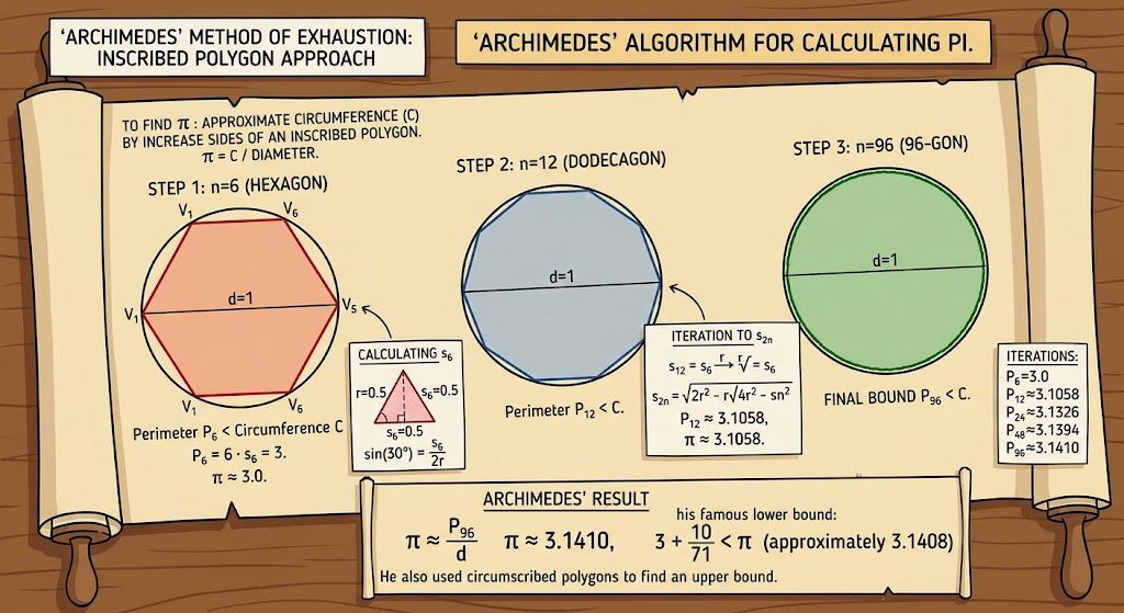
Another example of truncation error comes from Archimedes. Archimedes tried to approximate the circumference of a circle by inscribing a regular polygon with a finite number of sides. In a practical calculation or computer algorithm, you must stop at a finite number of sides, such as a 96-sided polygon. The truncation error here is the difference between the true perimeter of the circle ( ) and the perimeter of your finite n-sided polygon. By cutting off (truncating) the infinite increase of polygon sides, you miss a tiny bit of the curved boundary each time, leaving a gap between the straight edges and the true curve.

Have you ever wondered how a computer takes the real, continuous world and crams it into a digital file? The real world has infinite detail, but computer memory is limited. To make a digital copy, computers must chop reality along two different axes. This chopping creates two distinct types of mathematical errors: discretization error and quantization error.

Think of taking a photo of a sunset with a digital camera:

• Discretization Error (The Horizontal Axis): The camera sensor is divided into a grid of distinct squares called pixels. Discretization error is the loss of detail because you chopped continuous space into a grid. You lose whatever happens between the pixels—like a tiny star in the sky that falls right into the crack between two sensor squares. You can reduce this error by increasing your resolution (adding more megapixels).
• Quantization Error (The Vertical Axis): Once the camera picks a pixel square, it has to measure the exact color and brightness of the light hitting it. But the computer only has a fixed number of binary bits (like 8 bits, which allows for 256 color choices) to store that brightness value. If the actual brightness value is 154.673, the computer must round it to 155. Quantization error is this vertical roundoff error. It causes smooth sky gradients to break apart into distinct, ugly stripes called "color banding."

Discretization error is about where you look (cutting up time and space), while quantization error is about how accurately you measure what you see (rounding values to the nearest digital step). Together, they are the price we pay for turning the infinite universe into binary code!

Not all measurement errors behave the same way. Systematic error is an error that pushes your measurements consistently in the same direction. Imagine a bathroom scale that always reads 2 kg too high. If your actual mass is 60 kg, it might read 62 kg; at 70 kg, it might read 72 kg. Taking more measurements won't fix the problem—the scale itself is biased. Other examples include a ruler with a damaged or misplaced zero mark, a thermometer that consistently reads 2°C too high, or measuring the length of an object while always viewing the ruler from the same angle and introducing a consistent parallax error.

Random error is different: it causes measurements to vary unpredictably from one trial to the next. For example, when using a stopwatch to measure how long a ball takes to fall, your reaction time might cause you to start or stop the timer slightly early or late. You might measure 1.21 s, then 1.18 s, then 1.23 s. Other examples include tiny fluctuations in temperature or electrical signals, small changes in the position of an object, or slightly different readings when measuring the diameter of a pencil at different points.

Here's the key difference: systematic error tends to make all your measurements wrong in a similar way, while random error makes your measurements scatter around the true value. Repeating a measurement and averaging the results can reduce the effect of random error, but it won't fix a systematic error. To find systematic error, you have to find the source of the bias—and fix or account for it.

Error and uncertainty are related, but they are not the same thing.
Error is the difference between a measured or calculated value and the true or accepted value. If we measure a pencil as 7.24 mm and its true diameter is 7.26 mm, then the error is 7.24 - 7.26 = -0.02 mm, or 0.02 mm in magnitude.

The problem is that we usually do not know the true value, so we usually cannot determine the actual error directly. Instead, we estimate how much error might be present. This estimate is called uncertainty.

For example, if we report a pencil diameter as 7.24 ± 0.02 mm, the ±0.02 mm is an uncertainty. It tells us how much variation or error we believe is reasonably possible. It does not tell us the actual error. The actual error could be smaller, larger, positive, or negative—we simply do not know it.

In short: error describes the difference from the truth; uncertainty describes how unsure we are about our result.

What do you see in common with these examples?

• A computer program with different functions. If one function makes a calculation error, the output of the entire program is thrown off.
• An electric circuit with several components wired in series. If one component breaks down, the entire circuit stops working.
• Pretend you're building a 1500-ft tall skyscraper. A lot of modern towers use a reinforced concrete core, housing the stairs and elevators. This core acts as the vertical spine for the building. Now what if the walls at the foundation of the building are not exactly square to the foundation? In other words, instead of a 90° angle, what if the angle is 90.1°?
• Have you ever built a complicated Lego model? What happened when you made a mistake early on?

In every physical measurement, there is some degree of uncertainty—whether from the limits of your measuring tool or simple human estimation. But in science and engineering, measurements rarely exist in isolation. You plug them into equations, feed them into algorithms, or chain them together in physical systems.

When you perform mathematical operations on uncertain numbers, those initial uncertainties don't just stay the same; they combine, amplify, and pass forward through every step of the process. A slight misalignment in a ruler measurement can compound into a massive error when calculating volume, velocity, or structural stress. Understanding how error propagates lets you predict the reliability of your final result—and ensures a tiny mistake at the start doesn't completely wreck your outcome.

Both errors and uncertainties can be expressed in absolute or relative form.

Absolute error is the difference between a measured value and the true or accepted value, usually expressed as a positive magnitude:

Absolute uncertainty is the size of the uncertainty expressed in the same units as the measurement:

For example, in 7.24 ± 0.02 mm, the absolute uncertainty is 0.02 mm.

Relative error compares the absolute error with the measured value:

Relative uncertainty does the same thing with uncertainty:

Relative values are often written as percentages, which are dimensionless quantities. For example, an absolute uncertainty of 0.02 mm on a 7.24 mm measurement gives a relative uncertainty of approximately 0.28%.

When to use absolute vs. relative?

Absolute error or uncertainty tells you how much a quantity could be off, using the same units as the measurement. Relative error or uncertainty tells you how large that error or uncertainty is compared with the size of the quantity, usually as a percentage. Neither is universally better—the useful choice depends on what you are trying to understand.

Use absolute error or uncertainty when the actual size of the difference matters.
Absolute values are especially useful when you care about a physical limit, tolerance, or difference measured in specific units. Here are some examples:

• Machine tolerance: An engineer specifies that a shaft should be 10.00 mm in diameter, with a manufacturing tolerance of ±0.05 mm. The important question is whether the shaft is within 0.05 mm of the target—not what percentage of the diameter that represents.
• Measurement uncertainty: If a ruler measurement is 25.4 ± 0.2 cm, the 0.2 cm tells us directly how much uncertainty is associated with the measurement.

Use relative error or uncertainty when comparing quantities of different sizes.
A difference that is small in absolute terms can be enormous for a small quantity but insignificant for a large one. Relative error or uncertainty puts measurements on the same scale.

• Comparing two measurements: Suppose two measurements each have an uncertainty of 1 mm:
  • 10 mm ± 1 mm → 10% uncertainty
  • 100 mm ± 1 mm → 1% uncertainty
  Both measurements have the same absolute uncertainty, but the first measurement is much less certain relative to its size.
• Experimental results: Measuring the diameter of a large pipe to within ±1 mm might be excellent. Measuring a tiny electronic component to within ±1 mm might be completely inadequate. The relative uncertainty makes this difference obvious.

Remember: absolute and relative forms describe the same underlying error or uncertainty in two different ways. Absolute values are usually best when dealing with physical differences and tolerances; relative values are especially useful for comparing measurements and judging whether an error is large or small compared with the quantity itself.

Quiz // Question 1 OF 9

VIEW ALL SCORE: 0

When we use measured quantities in a calculation, their errors or uncertainties can affect the final result. How we combine them depends on whether we are considering a worst-case bound or a statistical estimate.

For a worst-case calculation, we assume that all errors or uncertainties happen in the direction that makes the final error as large as possible. For addition and subtraction, we therefore add the absolute uncertainties. For example:

10.0 ± 0.2 cm + 5.0 ± 0.1 cm = 15.0 ± 0.3 cm.

For multiplication and division, we instead add the relative uncertainties. For example, multiplying quantities with 2% and 3% relative uncertainty can give a result with as much as 5% relative uncertainty.

For powers, the same worst-case idea applies: if a quantity has a relative uncertainty of 2%, squaring it gives approximately 4% relative uncertainty, while cubing it gives approximately 6%.

These are worst-case rules. They are useful when we want a conservative bound on how large the error could be. When uncertainties come from independent random effects, however, we often use quadrature instead. In that case, we combine the contributions by taking the square root of the sum of their squares. For addition and subtraction, we combine absolute uncertainties in quadrature; for multiplication and division, we combine relative uncertainties in quadrature.

The key idea: addition and subtraction use absolute quantities; multiplication and division use relative quantities. Whether we add those quantities directly or combine them in quadrature depends on whether we are calculating a worst-case bound or a statistical uncertainty.

Operation	Worst Case Uncertainty	Statistical Uncertainty
Addition ( )
Subtraction ( )
Multiplication ( )
Division ( )

Quiz // Question 1 OF 22

VIEW ALL SCORE: 0

Whatever STEM field you pursue, you will eventually come across significant digits, a.k.a. significant figures. We'll first learn how to count the number of significant digits in a number, and then in the next section, we'll how to use significant digits to convey uncertainty. To count significant digits, we follow the following rules:

• Non-Zero Digits: Always count (e.g., 48.3 has three significant digits).
• Leading Zeros: Never count; they are just placeholders (e.g., 0.002 has one significant digit).
• Captive Zeros: Always count when trapped between non-zero numbers (e.g., 60.7 has three significant digits).
• Trailing Zeros: Count only if a decimal point is explicitly written (e.g., 500. has three, but 500 has only one).

Let's go through some examples:

Quiz // Question 1 OF 7

VIEW ALL SCORE: 0

Significant digits (sig figs) tell the reader how precisely a number has been reported. A measurement should not imply more precision than the instrument, method, or data can justify. If you use a cheap plastic ruler, your data shouldn't look like it came from a million-dollar laser. Extra digits do not create extra information—they create the illusion of precision.

Rules for using significant digits in measurements:

• Rule 1: Assume the uncertainty is ±1 in the last significant place.
• Rule 2: The Uncertainty Dictates the Value
  When reporting a measurement with a ± uncertainty, the uncertainty determines how precisely the value should be reported. For this course, use this two-step rule:
  
  1. Round the uncertainty to one significant digit.
  2. Round the measured value to the same decimal place.
  Bad: 12.347 ± 0.263 cm
  Good: 12.3 ± 0.3 cm
  Why? The uncertainty 0.263 cm rounds to 0.3 cm, which is precise only to the tenths place. Therefore, the measured value must also be rounded to the tenths place: 12.3 cm.
• Rule 3: Calculations Are Limited by the Input Data
  When you combine measurements, your calculation should not produce a final answer that appears more precise than the least precise input. The calculation determines the numerical result; significant-digit rules determine how that result should be reported.
  
  Addition & Subtraction → Count Decimal Places
  The result should not have more decimal places than the quantity with the fewest decimal places.
  
  Example:
  15.1 cm + 2.03 cm = 17.13 cm → 17.1 cm
  
  The first measurement is known only to the tenths place, so the answer is reported to the tenths place.
  
  Multiplication & Division → Count Significant Digits
  The result should not have more significant digits than the quantity with the fewest significant digits.
  
  Example:
  5.0 cm x 3.00 cm = 15.0 cm² → 15 cm²
  
  The first measurement has only two significant digits, so the answer is reported with two significant digits.

The Takeaway: Significant digits are about honesty in communication. They keep us from reporting digits that our measurements or calculations do not justify. They do not make a measurement more accurate, and they do not tell us how close we are to the true value—they simply make sure that the precision we communicate matches the information we actually have.

Quiz // Question 1 OF 14

VIEW ALL SCORE: 0

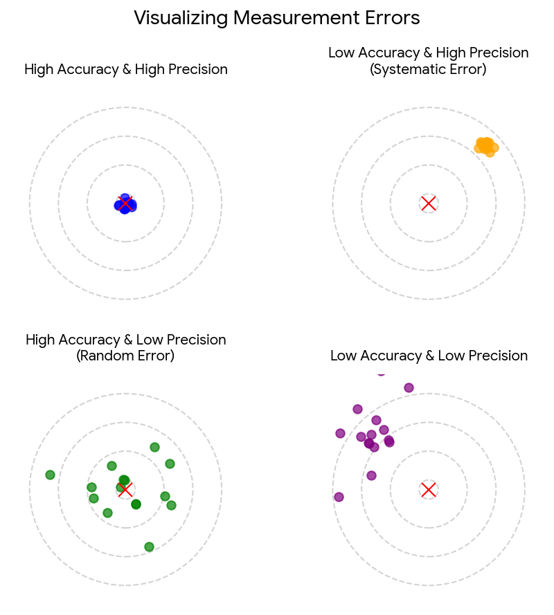
Two measurements can be “good” in very different ways. Accuracy describes how close a measurement is to the true or accepted value. Precision describes how closely repeated measurements agree with each other. In other words, accuracy is about hitting the target; precision is about hitting the same place repeatedly.

Imagine measuring the diameter of a pencil five times. If your measurements are 7.21, 7.22, 7.21, 7.22, and 7.21 mm, they are precise because they are tightly grouped. But if the pencil's true diameter is 7.50 mm, they aren't very accurate. On the other hand, measurements of 7.48, 7.53, 7.49, 7.51, and 7.50 mm are both accurate and reasonably precise—even though they aren't all exactly the same.

The important lesson is that precision does not guarantee accuracy. You can make the same wrong measurement over and over again. A well-calibrated instrument and a good measurement technique help you achieve both: measurements that are close to the true value and consistent from one trial to the next.